Overview

In this project, I implemented the following:

  1. Run edge detection for images using the finite difference operator and the derivative of gaussian (DoG) filter
  2. Sharpen images (and blur then re-sharpen images)
  3. Create hybrid images in the SIGGRAPH 2006 paper by Oliva, Torralba, and Schyns
  4. Embark on the oraple journey for multi-resolution blending

the (in)famous oraple


Part 1: Fun with Filters

2D convolutions and filtering

Part 1.1: Finite Difference Operator

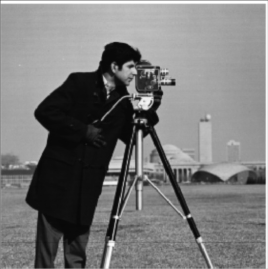
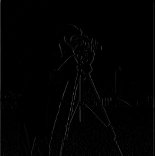
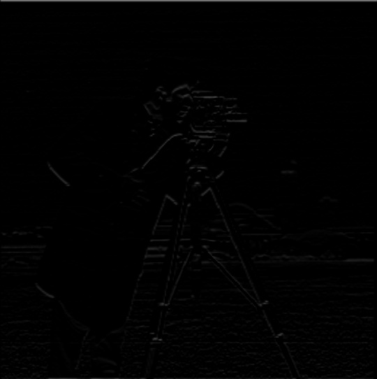
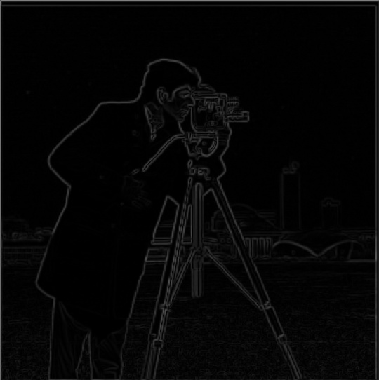
In this part, we use the finite difference operator to do edge detection of our cameraman image. We convolve the Dx and Dy arrays with our cameraman image to compute the "partial derivatives" of our image in the X and Y directions. Then, we take the square root of the sum of the squares of the partials to achieve the gradient of the image.

D_x and D_y

Partial Derivative

The gradient image

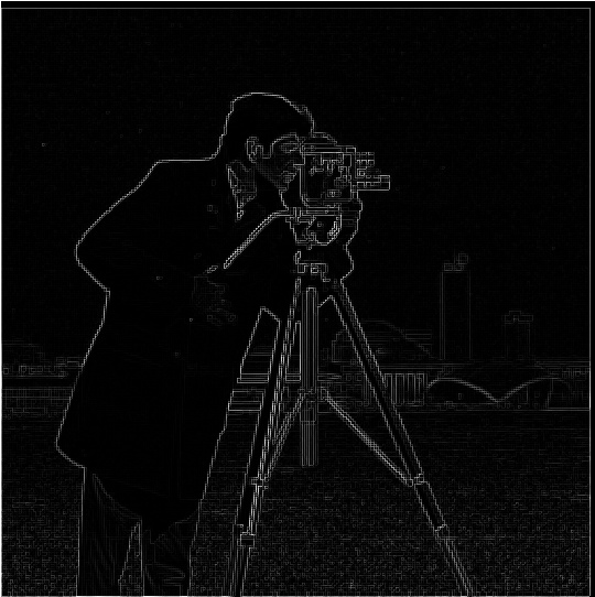
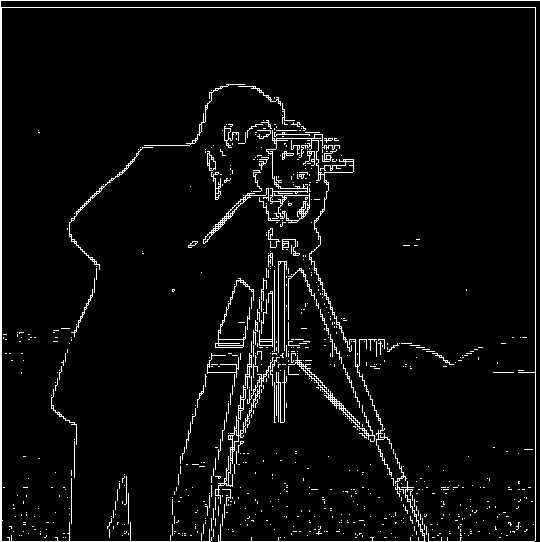
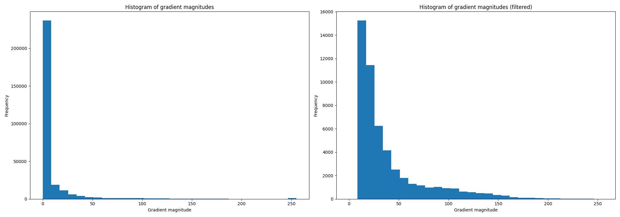
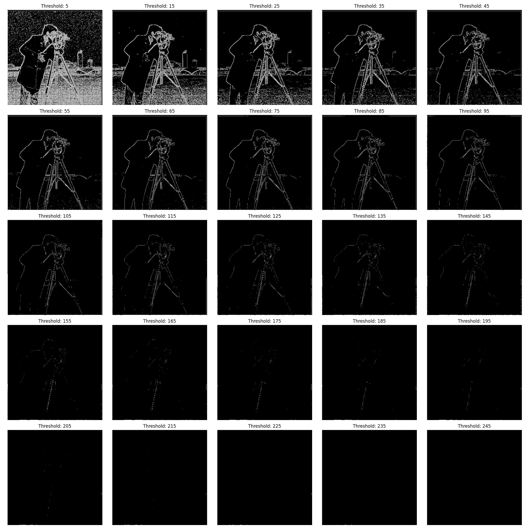
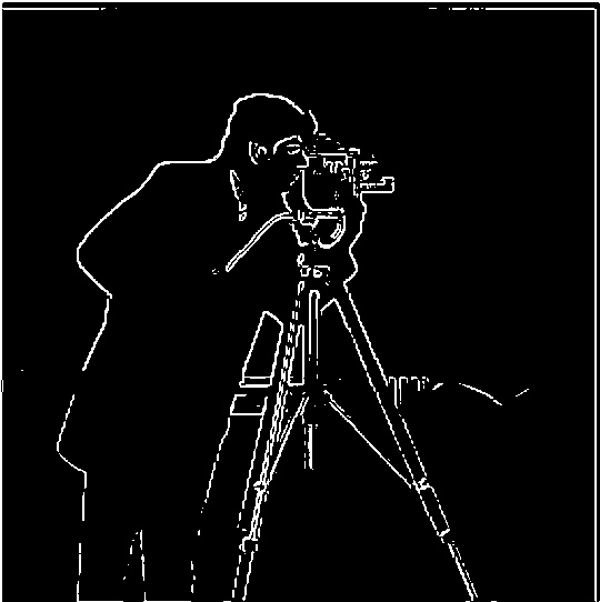
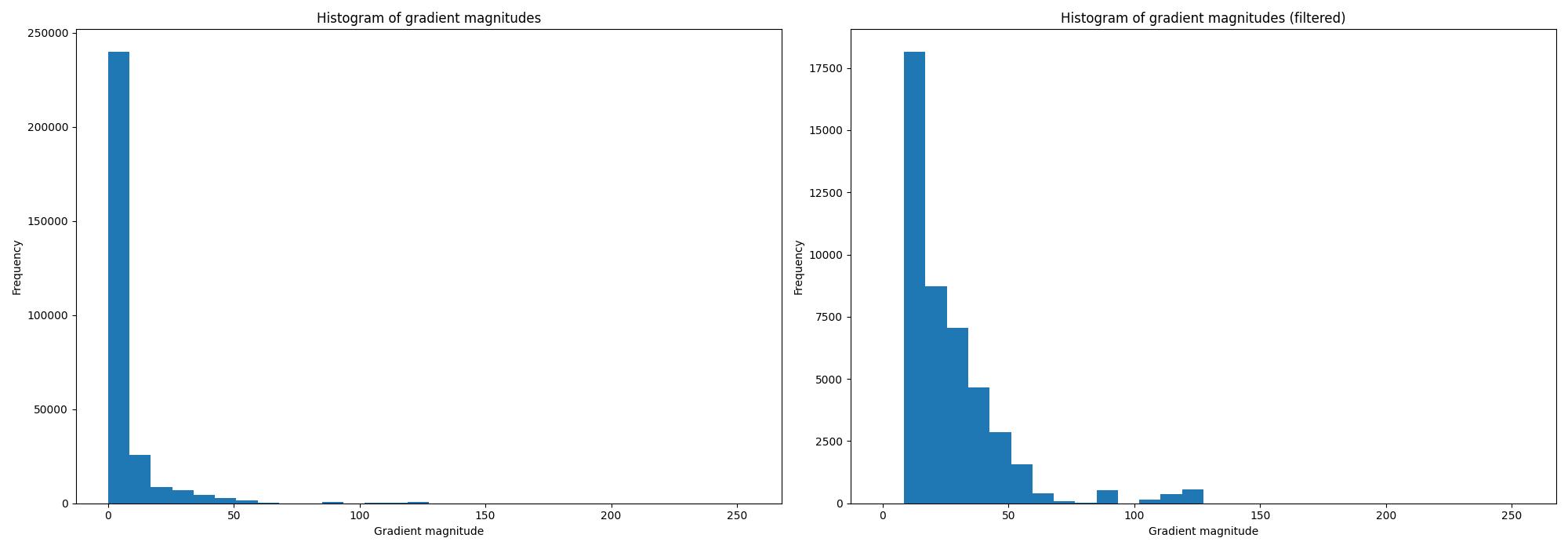
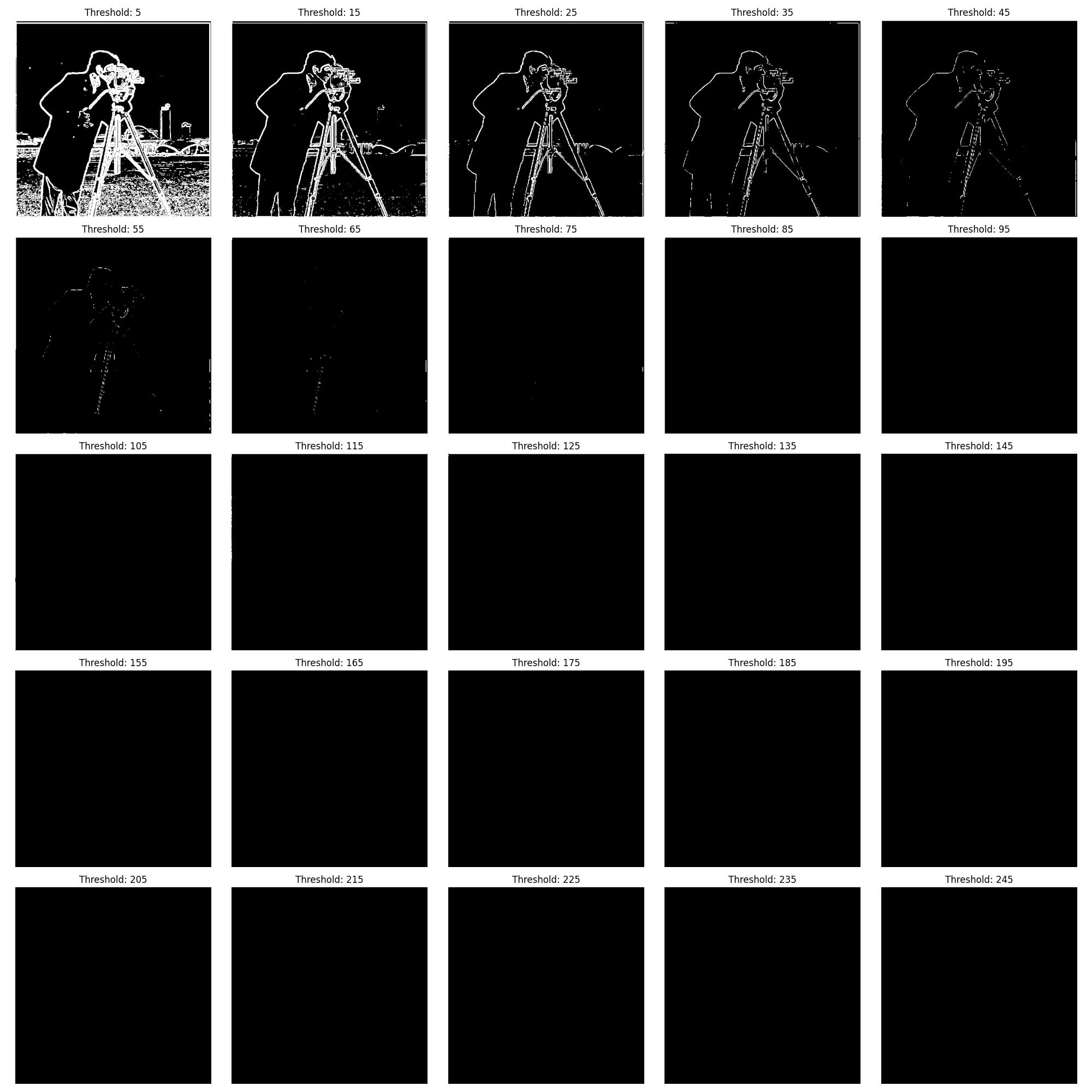
Down below, we display the partial derivatives, the gradient, and binarized gradient after it's been thresholded. I chose the threshold to be 50 (out of 255) by inspection and by viewing the distribution of the gradient magnitudes via a histogram.

Cameraman dX

Cameraman dY

Cameraman gradient magnitude

Cameraman gradient binarized

left: full histogram of the cameraman gradient
right: same histogram as the left but only keeping values between 10 and 250 for better viewing.

The cameraman gradient image at different thresholds (5-245 in increments of 5)


Part 1.2: Derivative of Gaussian (DoG) Filter

As we can see from the binarized image, simply using the difference operator yields noisy results. Thus, we need to use Gaussian filtering as a smoothing operator to reduce the noise. We accomplish this by taking 2 approaches that ultimately yield the same result:
(1) Convolve the cameraman image with a Gaussian filter and then apply the difference operator
(2) Convolve the cameraman image with two derivative of Gaussian filters (one for each of X and Y)

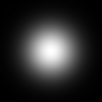
Gaussian Filter

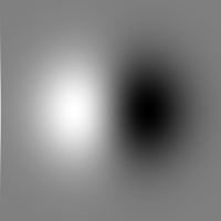
DoG, dX

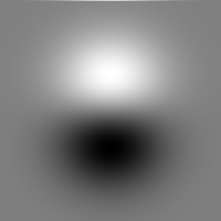
DoG, dY

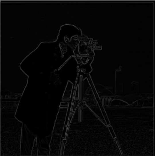
We use the Gaussian filters above to convolve and create our images. The first approach convolves the image with our Gaussian filter and then convolves the blurred image with the Dx and Dy difference operators to compute the gradient. The second approach has fewer operations in the sense that the image convolves directly with the difference of Gaussian filters to compute the gradient. By visual inspection, we can see that the resultant gradients from both approaches are the same.

Cameraman blurred

Cameraman blurred dX

Cameraman blurred dY

Cameraman blurred gradient (approach 1)

Cameraman blurred gradient (approach 2)

Cameraman blurred gradient binarized (using approach 1's image)

Some differences we can see is that the the resulting images using the Gaussian filter are smoother and less noisy as opposed to the images generated by using the finite difference operator. We can also see that the pixel values/intensities are lower in the blurred gradient as compared to the gradient from the difference operator. This is because the Gaussian filter is a low-pass filter that reduces the high frequency noise in the image. Another thing we can observe is that the edges are thicker than before, which makes sense given that we have blurred and therefore have "spread out" the effects of the edge. Otherwise, the threshold for creating the binarized image was done via inspection once again, set to 32 (out of 255) this time.

left: full histogram of the blurred cameraman gradient
right: same histogram as the left but only keeping values between 10 and 250 for better viewing.

The cameraman gradient image at different thresholds.


Part 2: Fun with Frequencies

image "sharpening" and hybrid images

Part 2.1: Image "Sharpening"

In this part, we use the unsharp masking technique to sharpen an image. We accomplish this by taking getting the high frequences of the image (by subtracting the blurred image from the original), scaling it up by some alpha, and adding it back to our original image. Here is what the equation looks like (g is the Gaussian filter):

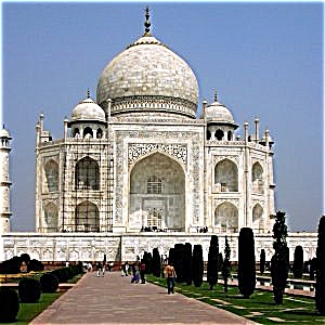
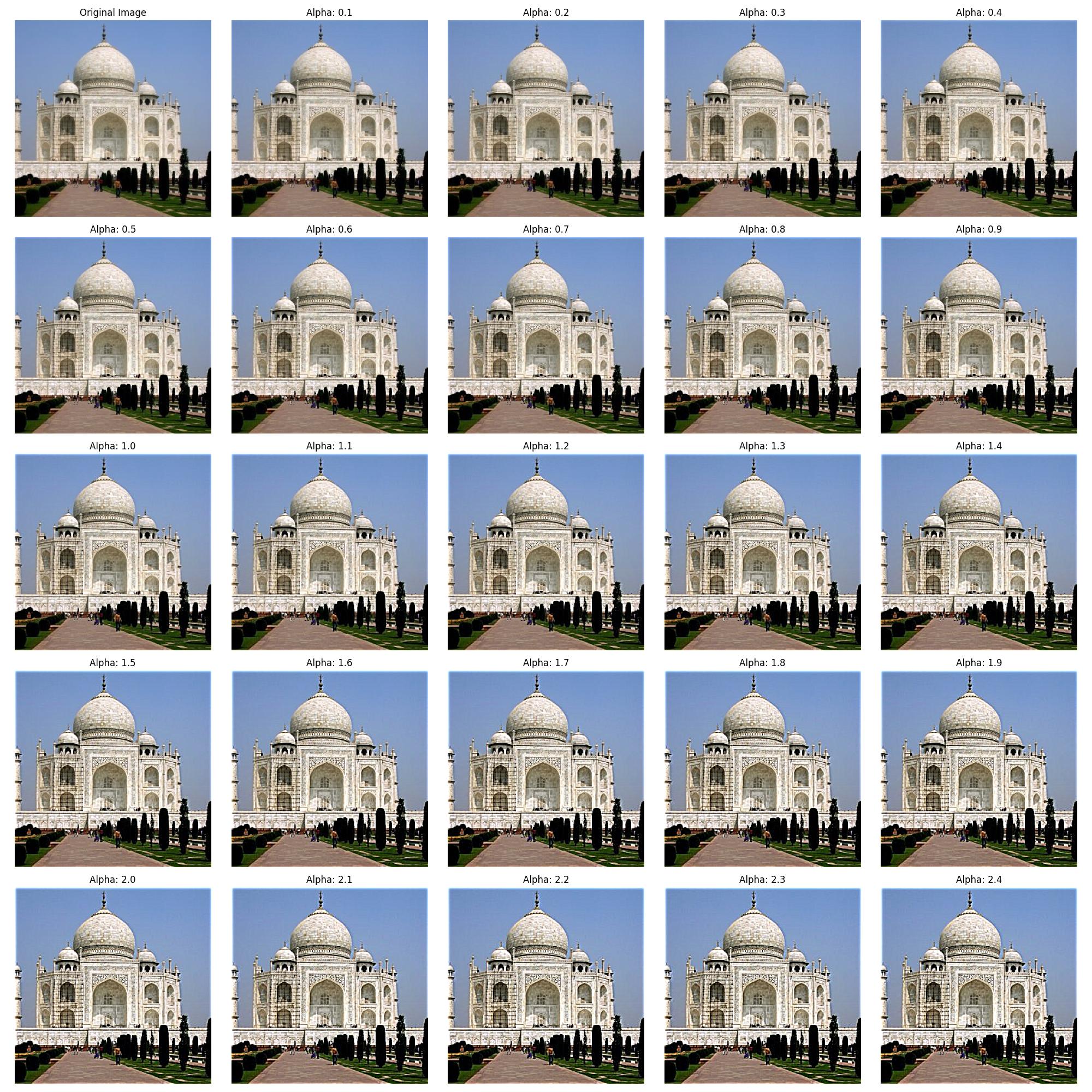
First up, we have the original Taj Mahal image, the sharpened Taj Mahal image (alpha=2), and a grid that shows the sharpened images of the Taj Mahal at various values of alpha.

Original Taj Mahal

Sharpened Taj Mahal

Grid of sharpened Taj Mahals

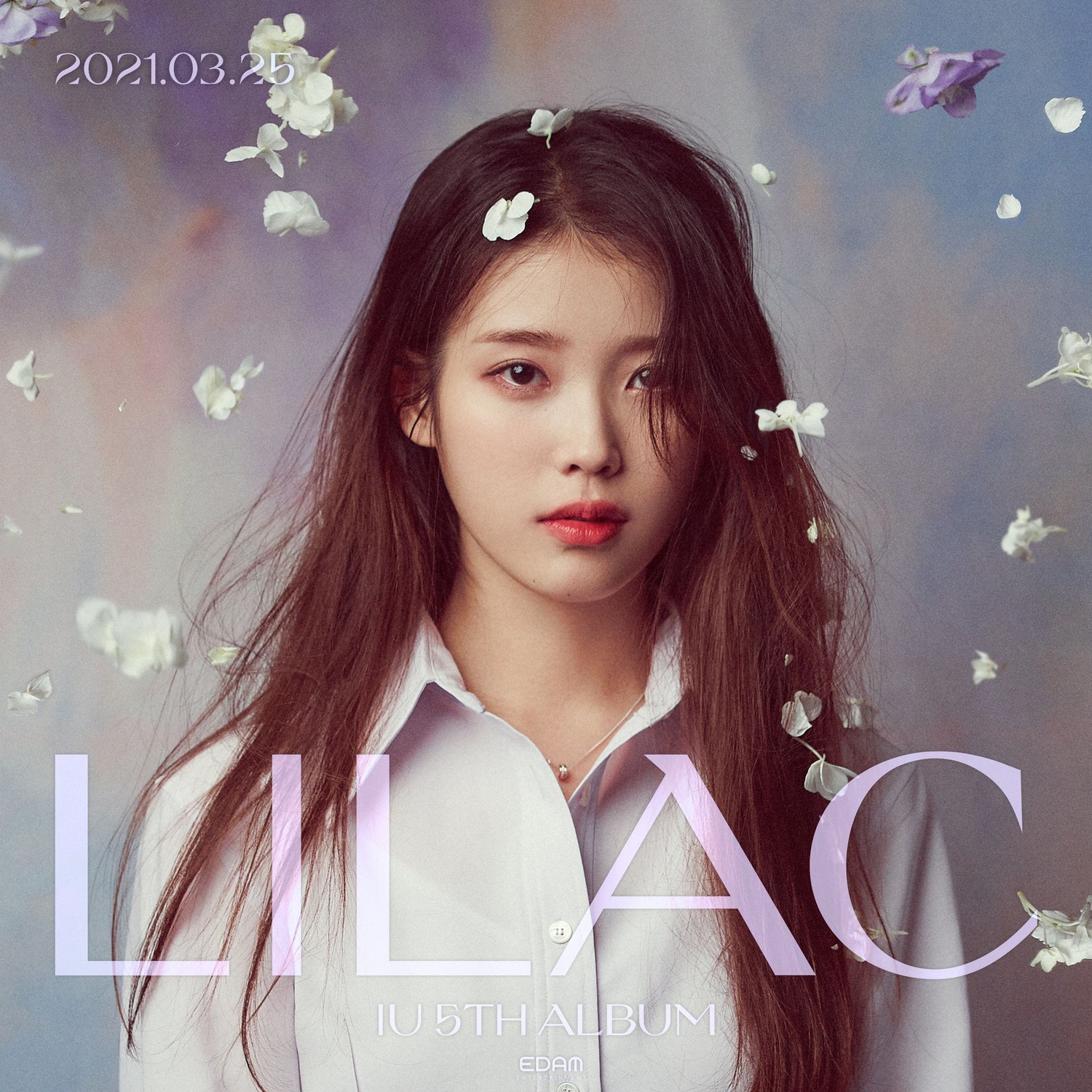
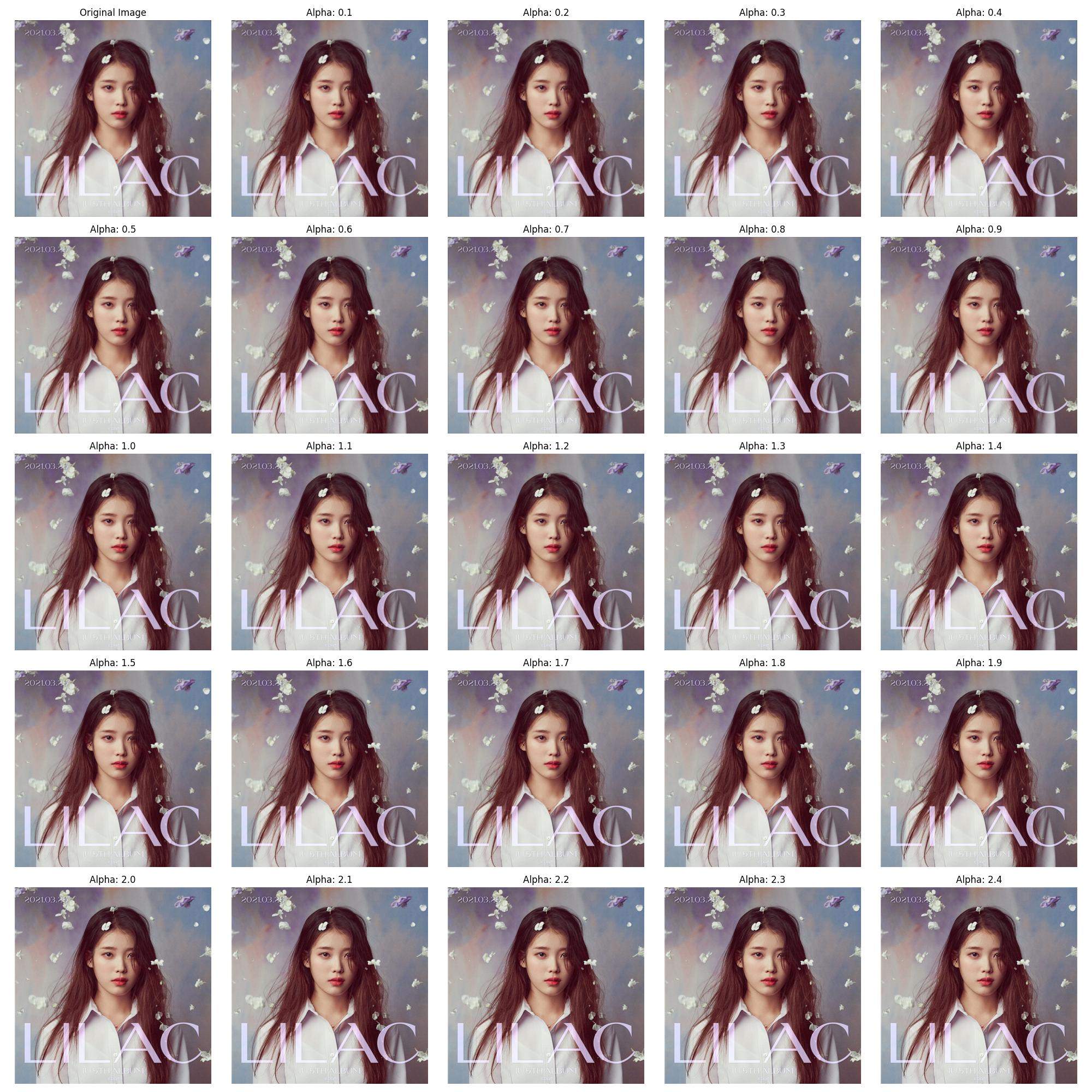
This second set of images with IU is more or less the same as above, but with the blurred version of the original image that we then use to re-sharpen (alpha=2). To see the effects of blurring and sharpening for the IU image, we can focus on her eyes and see the difference in sharpness (and can zoom in to observe affects better as well). Although the sharpened image of the blurred image isn't as sharp as the original, we can clearly see differences in sharpness between the blurred and the sharpened images.

Original IU

Blurred IU

Blurred IU sharpened

Grid of sharpened blurred IUs

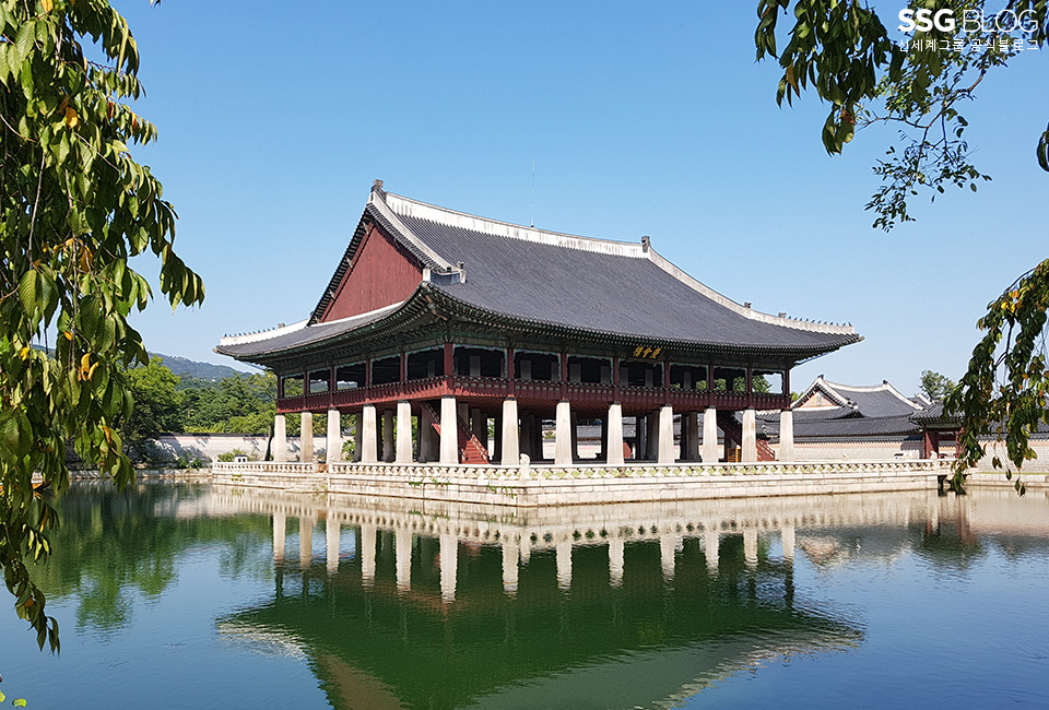
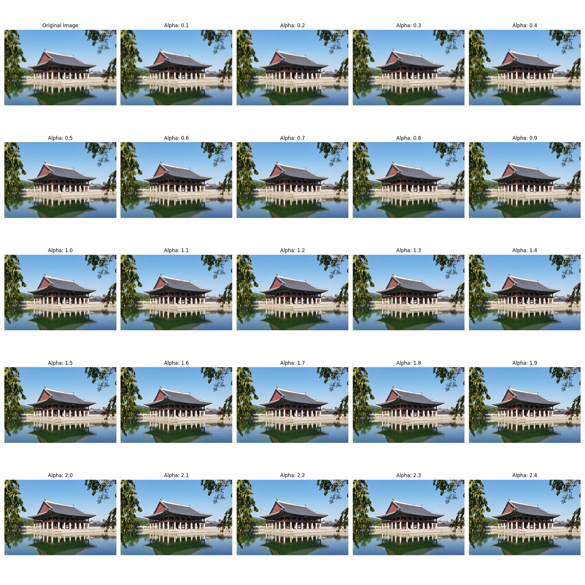
We do the same thing as above with the Gyeonghoeru Pavilion as we did with IU. This time around, we had to set the alpha much higher than the previous two (alpha=4) to make the image somewhat clear; this may be due to the fact that the blurred image is quite blurred, thus causing us to be missing a lot of high frequency information.

Original Gyeonghoeru

Blurred Gyeonghoeru

Blurred Gyeonghoeru sharpened

Grid of sharpened blurred Gyeonghoeru Pavilions


Part 2.2: Hybrid Images

In this part, we attempt to create hybrid images using the approach described in the SIGGRAPH 2006 paper by Oliva, Torralba, and Schyns. We accomplish this by taking two images, aligning them, and passing each image through either a high-pass or a low-pass filter. Then, combining the high-frequency details of one image with the low-frequency components of another creates a hybrid image, which is perceived differently depending on the viewing distance.

Down below, we have three sets of images. This first set is Derek and Nutmeg, the second set is Irene and Seulgi (with the corresponding Fourier analysis), and the third set is Trump and a bald eagle.

Derek aligned and low-passed
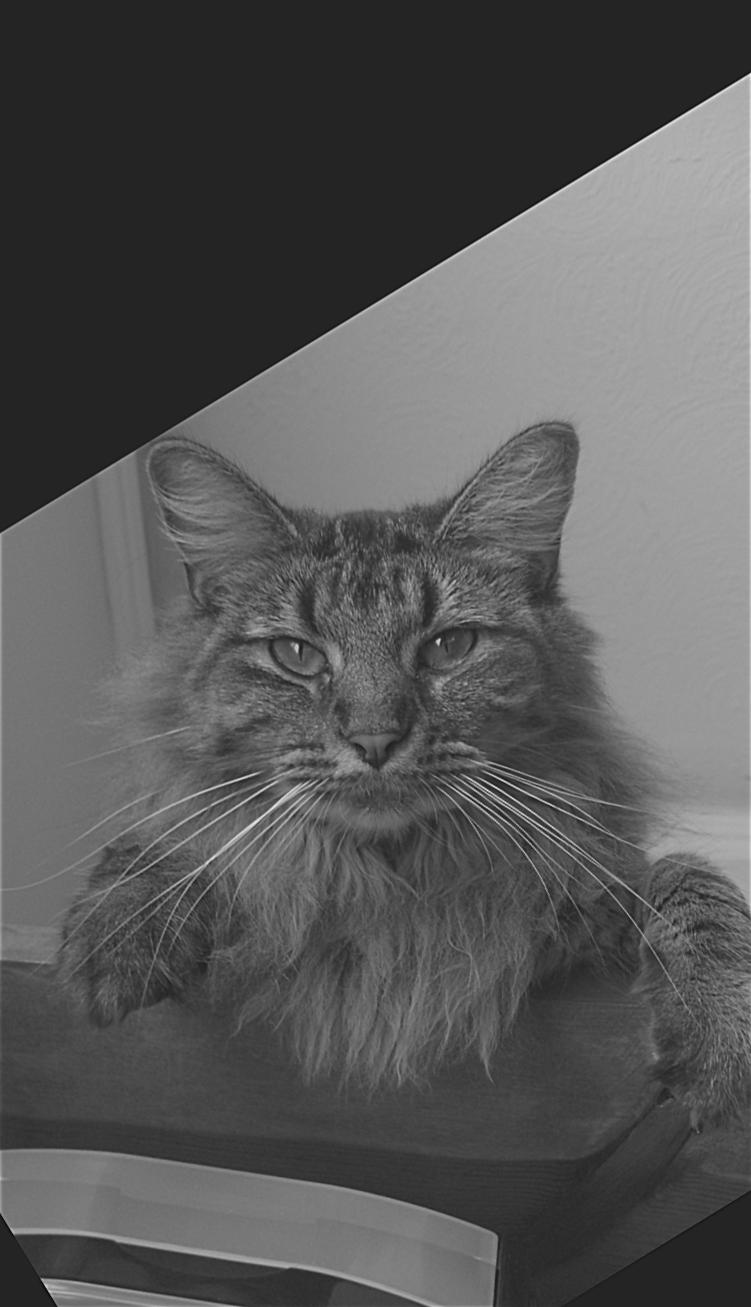
Nutmeg aligned and high-passed
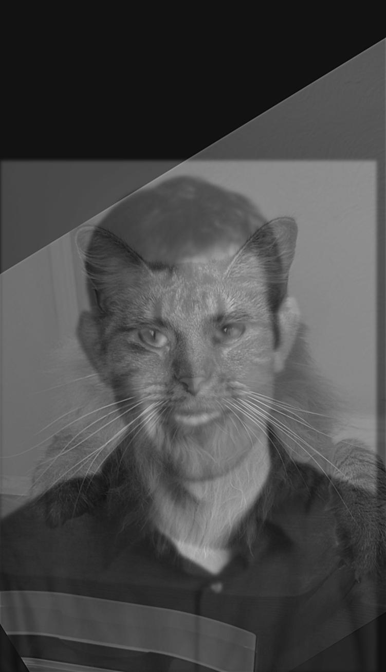
Dermeg hybrid image (Derek + Nutmeg)

Here is my favorite hybrid image, which is between Irene and Seulgi (aka Seulrene). Down below, we can see the low-pass image, high-pass image, hybrid image, and their corresponding Fourier analysis. The photos are from Red Velvet's Summer Magic EP, and the resultant image is Seulrene. Given all of the Seulrene ships all these years, I am happy to see that the hybrid image works pretty nicely.
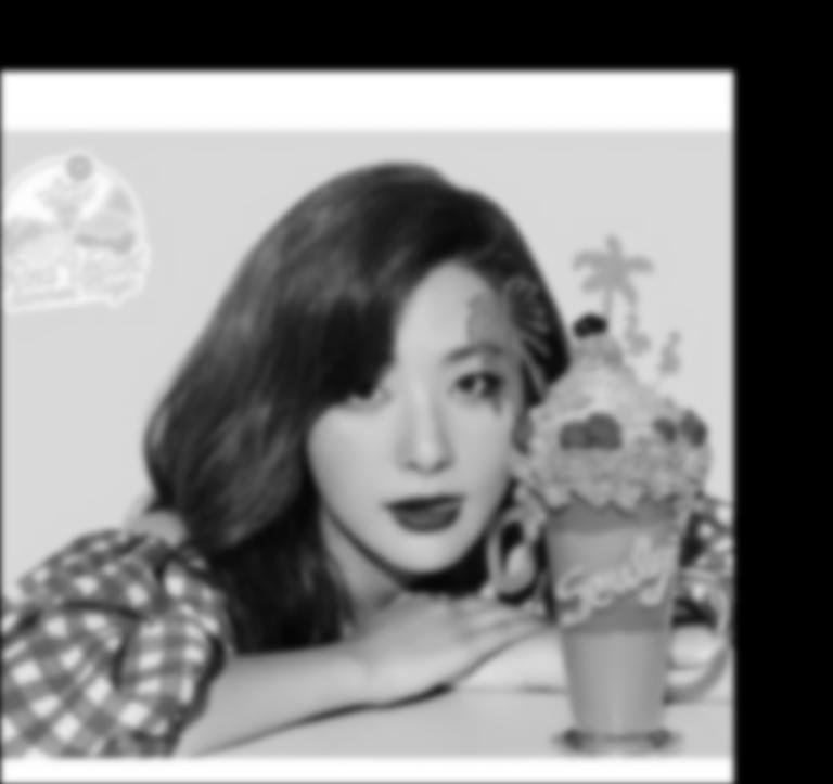
Seulgi aligned and low-passed
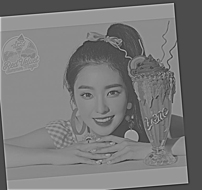
Irene aligned and high-passed
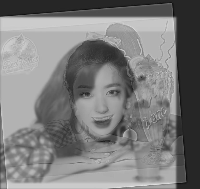
Seulrene hybrid image (Seulgi + Irene)
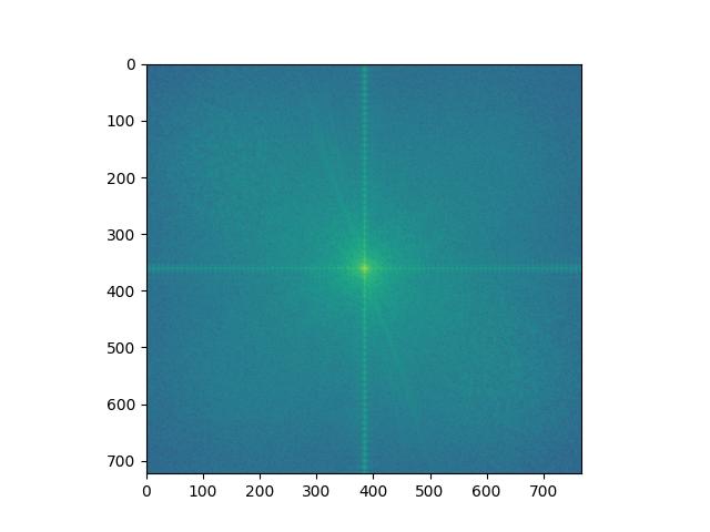
Seulgi aligned and low-passed FFT analysis
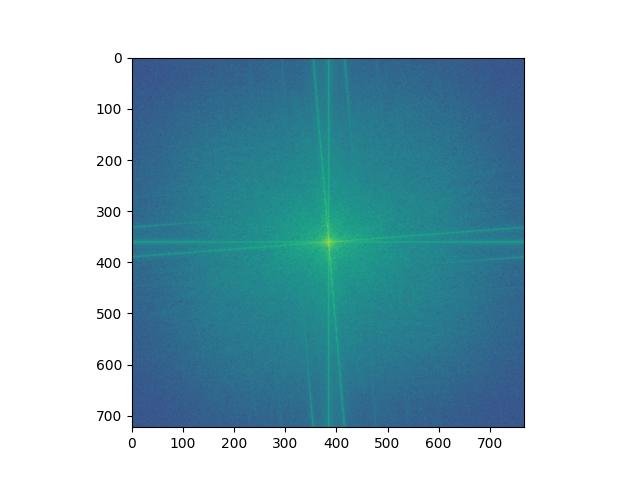
Irene aligned and high-passed FFT analysis
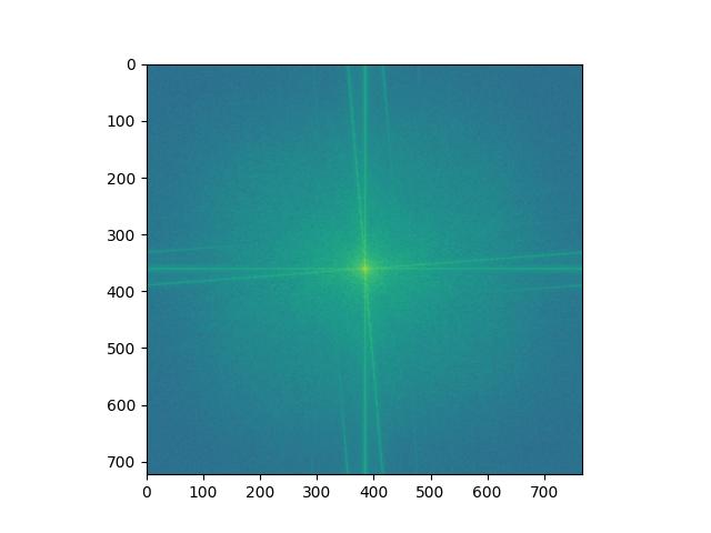
Seulrene hybrid image FFT analysis

Last but not least, we have a blend between Trump and a bald eagle, which I have aptly named "freedom". This one doesn't seem to work as nicely as the other images despite trying various different levels of filter size and alpha. This is probably due to the fact that both images are fairly high frequence and the general outline of the images generally differ as well.
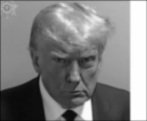
Trump aligned and low-passed
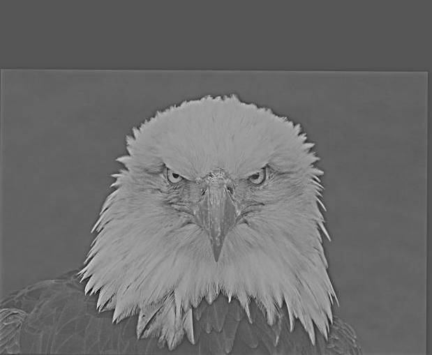
Bald eagle aligned and high-passed
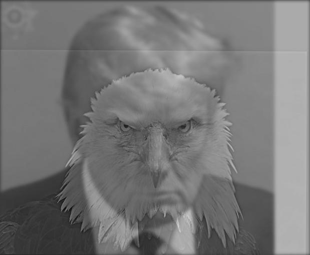
Freedom hybrid image (Trump + bald eagle)


Part 2.3: Gaussian and Laplacian Stacks

In this part, we implement the Gaussian and a Laplacian stacks. I first computed the Guassian stack by continually blurring the original image; as we go down the stack, we increase the sigma so that the image gets more blurred. As for the Laplacian stack, we take the difference between consecutive elements in the Gaussian stack with the last element being the same as the last element in the Gaussian stack.
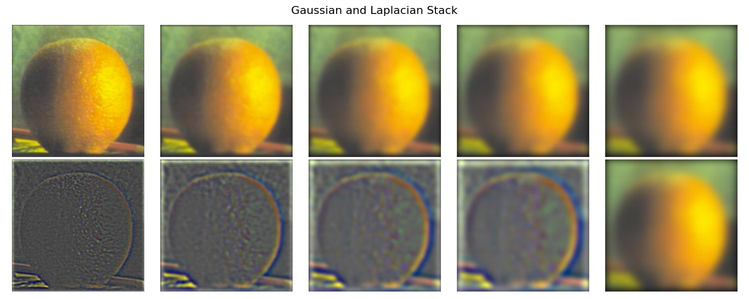
Gaussian and Laplacian stacks for orange
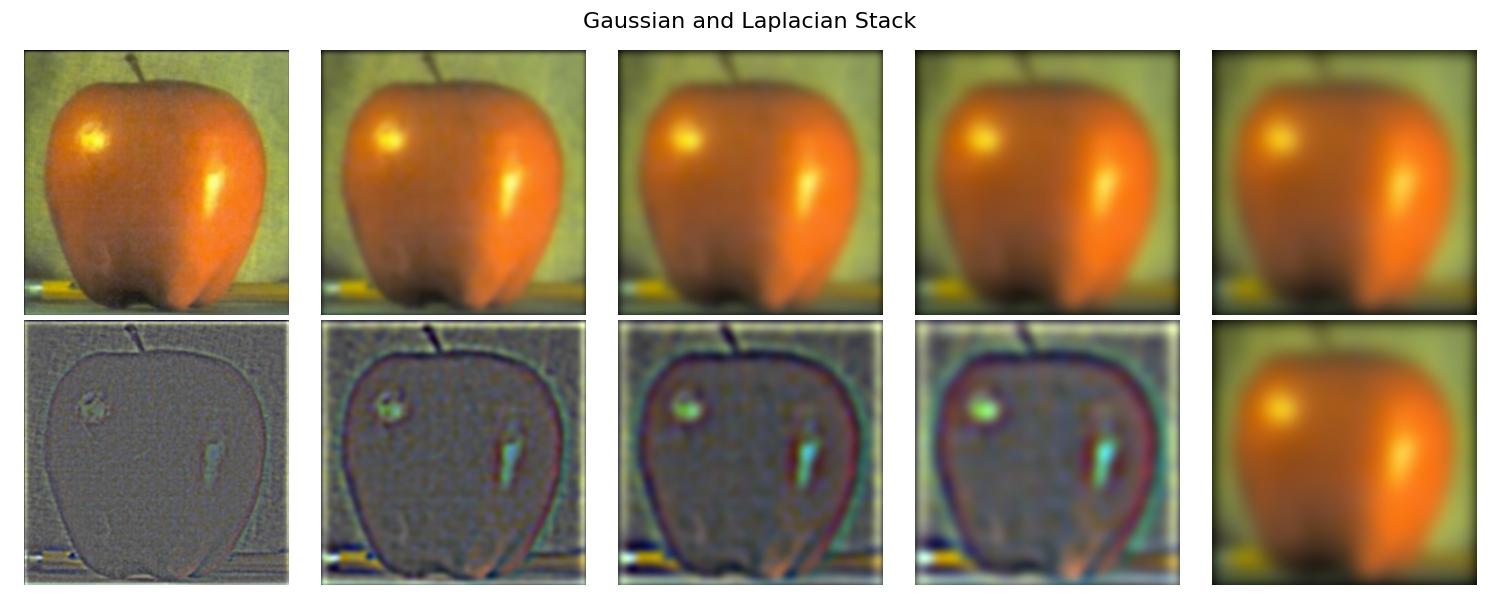
Gaussian and Laplacian stacks for apple


Part 2.4: Multiresolution Blending

We have finally reached the part of the project that has the oraple. In this part, we utilize the Gaussian and Laplacian stacks from part 2.3 to do multiresolution blending. In each row, we will show the two images that were used, the mask, and the final blended image.

Orange + Apple = Oraple
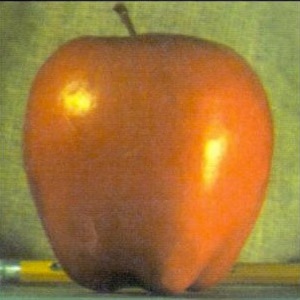
Apple
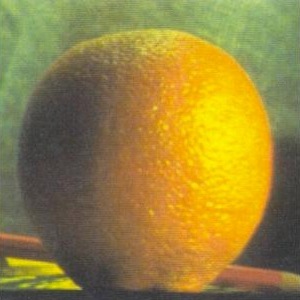
Orange

Oraple mask
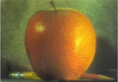
Oraple

Campanile + Hoover = Hoovernile
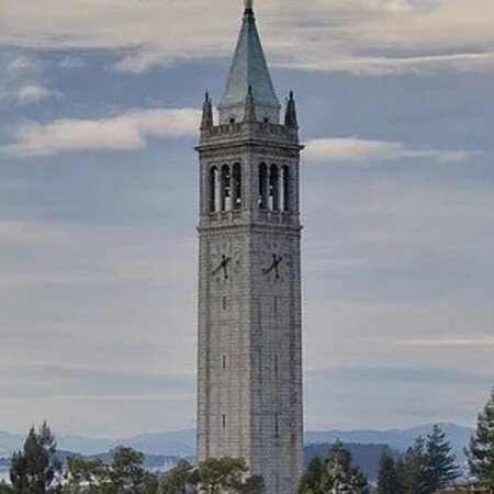
Campanile
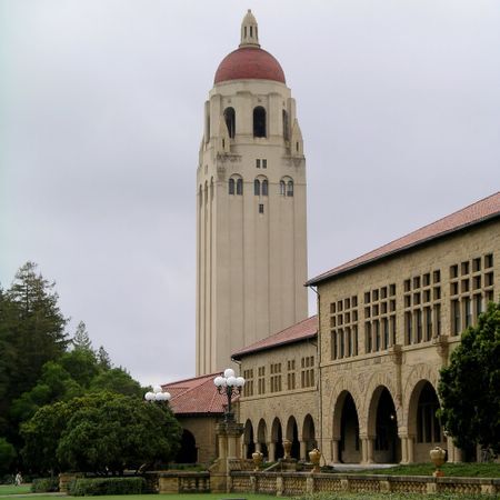
Hoover
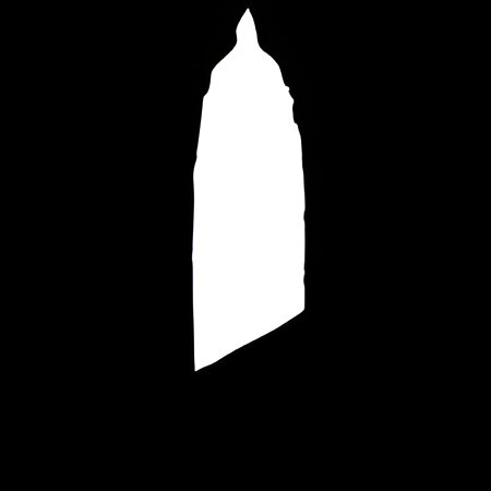
Towers mask
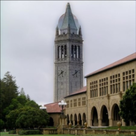
Hoovernile

Red Bull (RB19) + Mercedes (W13) = Silver Wings
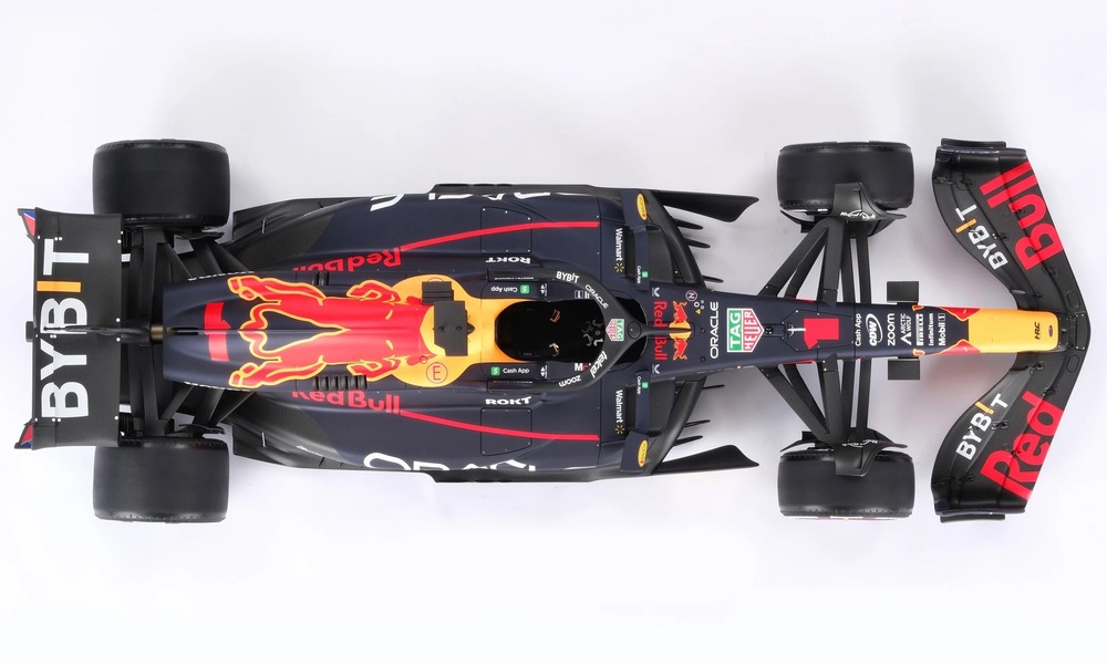
Red Bull
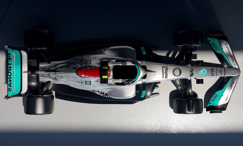
Mercedes

F1 mask
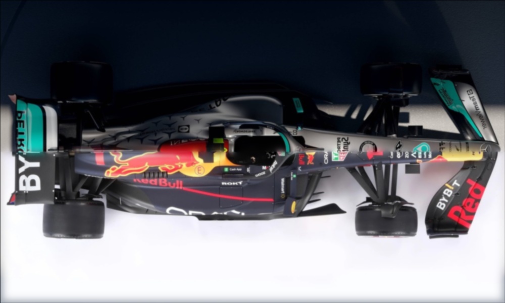
Silver Wings

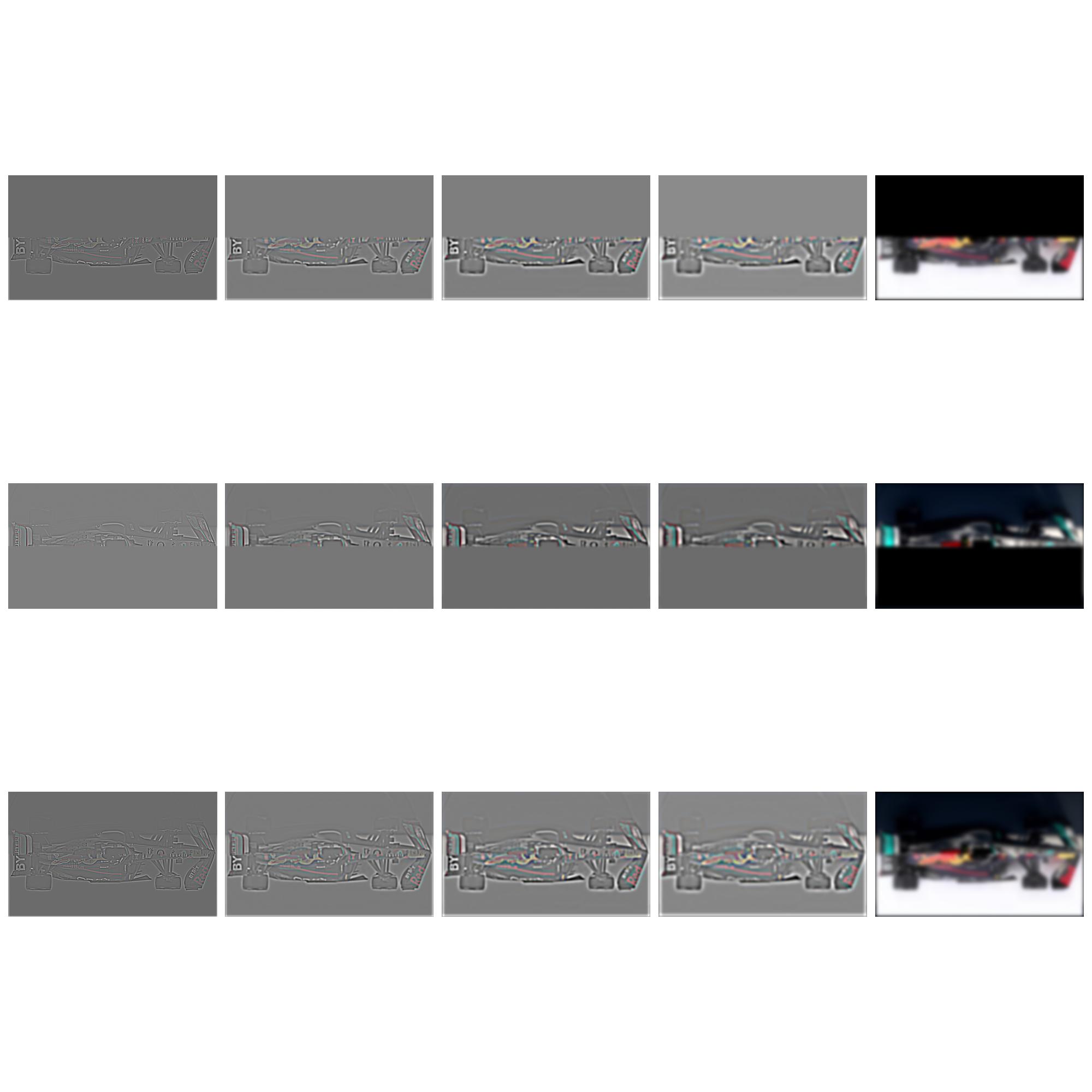
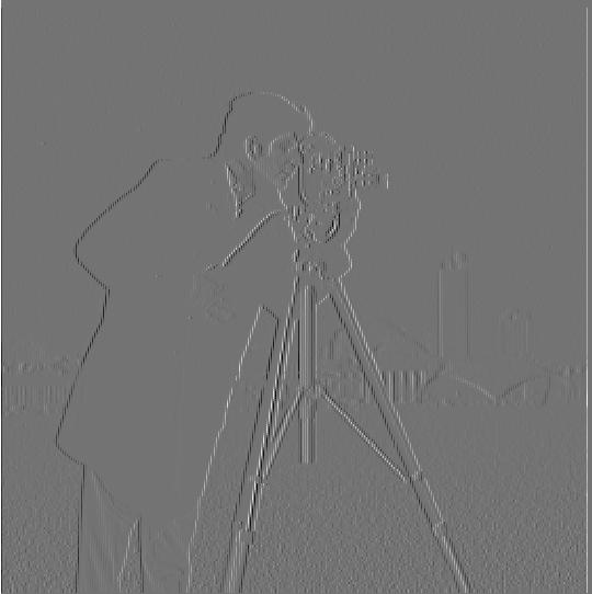
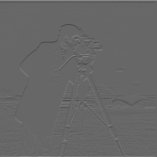
My favorite blending is the one for Silver Wings, so here are the Laplacians stacks for the masked input images and the resultant blended image.

Reflection + Acknowledgements

Reflection

My key takeaway is learning how to transform images using frequency analysis. Although I’ve learned about signal processing and frequency analysis in the classroom, this is my first time applying this theory in practice. It was pretty cool to see how we can implement frequency-based methods to blend images and utilize basic techniques to create effects commonly seen in photo editing software, almost fully from scratch.


Acknowledgements

This project is part of the Fall 2024 offering of CS180: Intro to Computer Vision and Computational Photography, at UC Berkeley. This website template is modified from HTML5 UP, and the images are from various sources from Google.